1 - Sisotool

We are now designing the PID controller for G(z). The fisrt step is to open Sisotool, go to the Root Locus Diagram and add two poles, one in 0 and another in 1, and then two zeros in between the poles.

After adding the zeros, you will move them in order to make the system to converge to its final value in the fastest way possible, that is, making sure the branches of the RLD are closer to the center of the unitary circle.

Finally, you will move the pink dot (compensator) along the branch. You should get to a point thats colsest to the center of the unitary circle. That way, you'll obtain all necessary data for the next step.

To open Sisotool, type:

sisotool(Gz) % Opens Sisotool using Gz for every plot

You should see the RLD, something similar to Figure 1.

Figure 1. Root Locus Diagram of G(z) before the manipulation

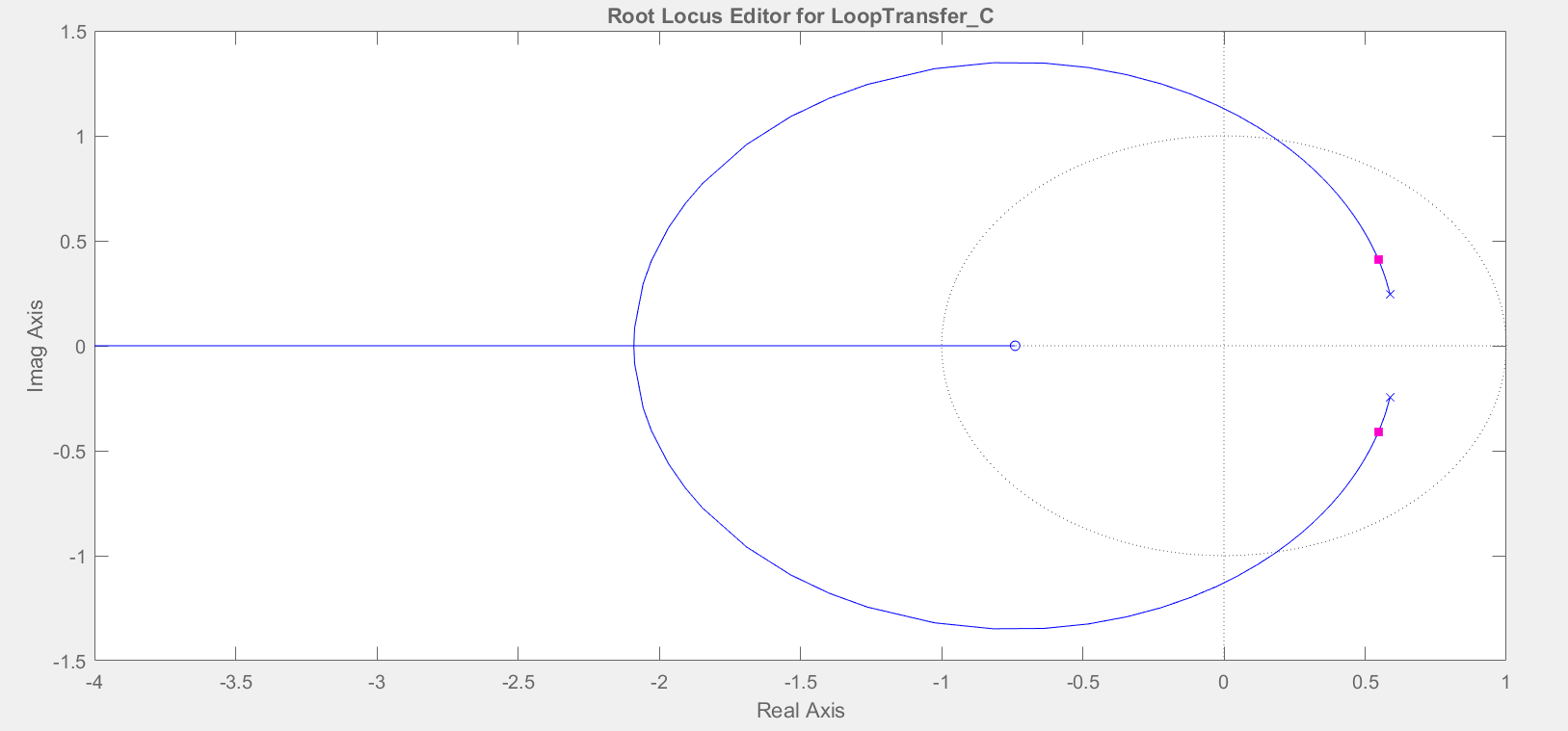
Figure 2. Adding zeros and poles to the RLD. The X shaped icon is a pole, the O shaped one is a zero.

You should place two poles, one at 0 (center of the unitary circe) and the other at 1. Then, add two zeros in between the poles you just added.

NOTE: You can edit a zero/poles position on Edit Compensator (Right-click over a blank area > Edit compensator)

Figure 3. RLD after adding two poles and two zeros.

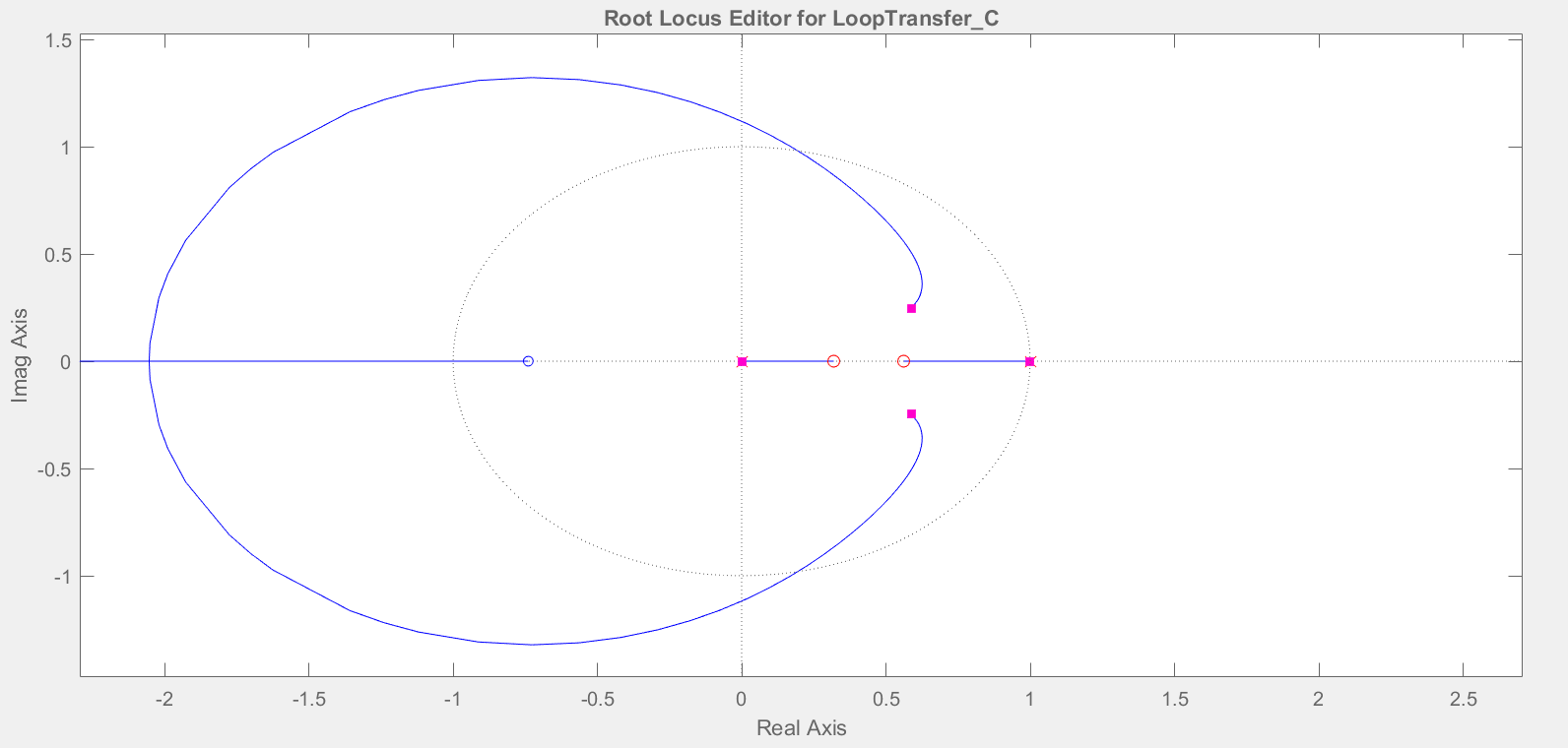
Figure 4. RLD after manipulating the zeros. Notice how the branches are now closer to the center of the unitary circle.

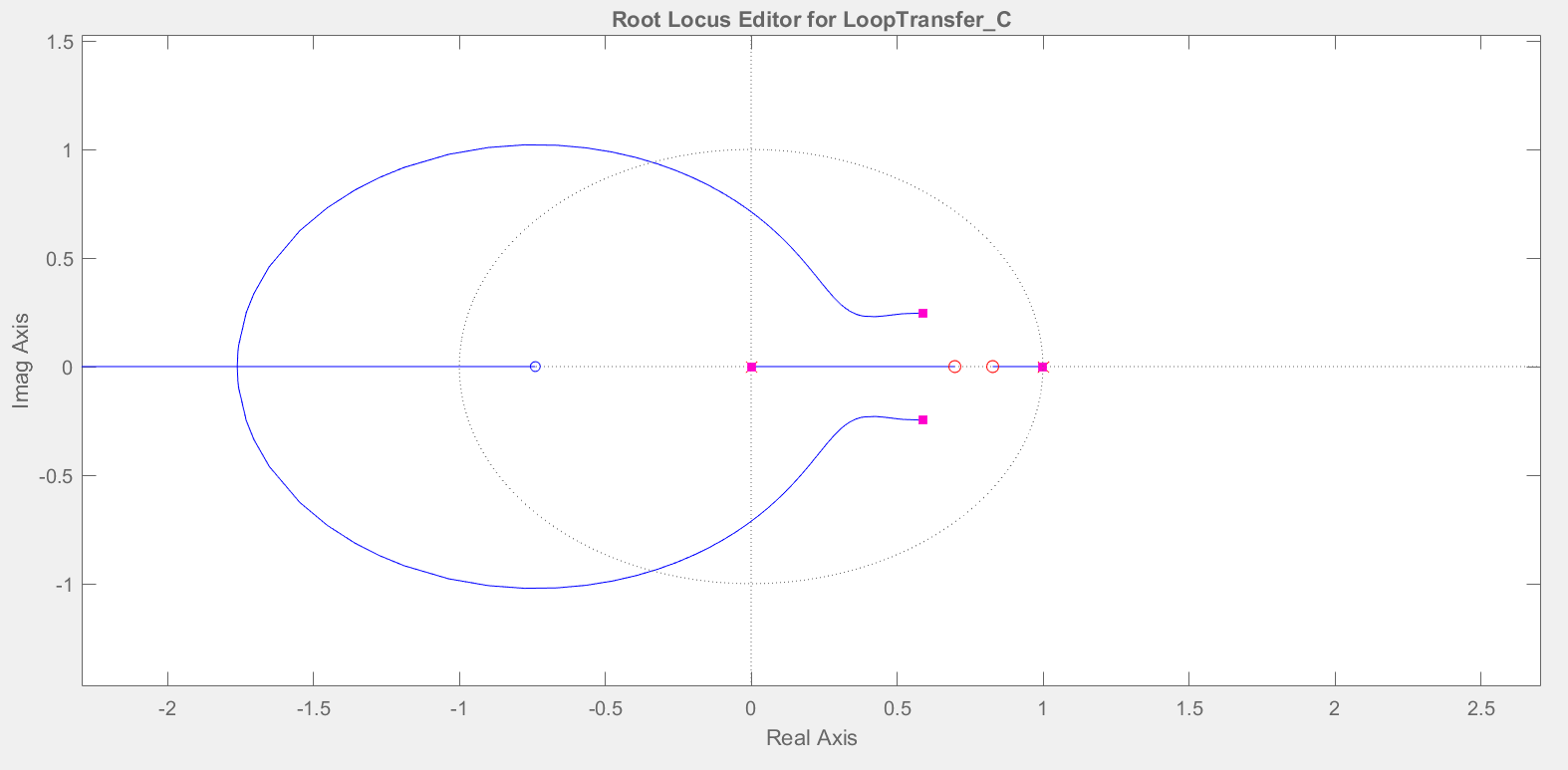
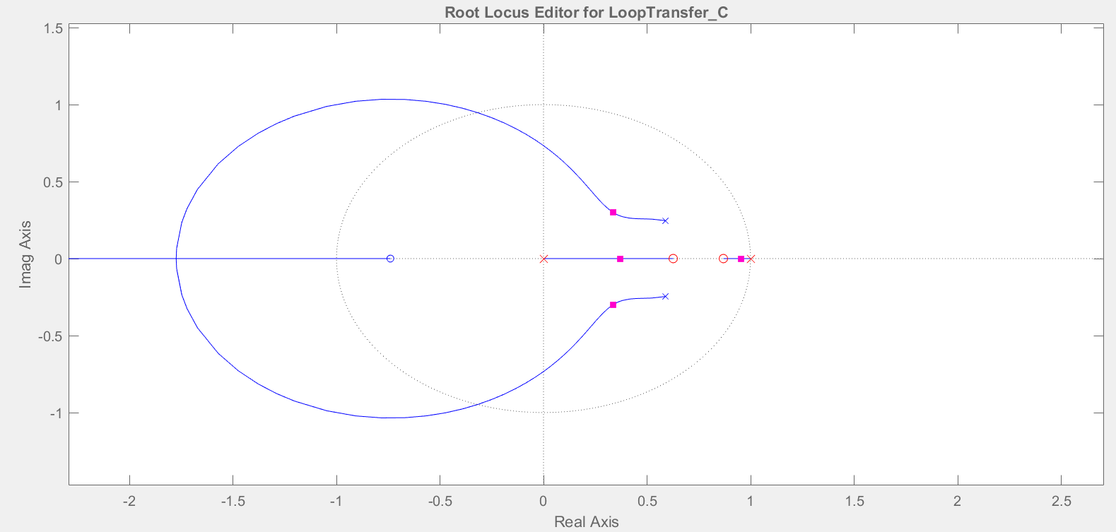
Figure 5. RLD after moving the pink dot to the nearest point from the origin.

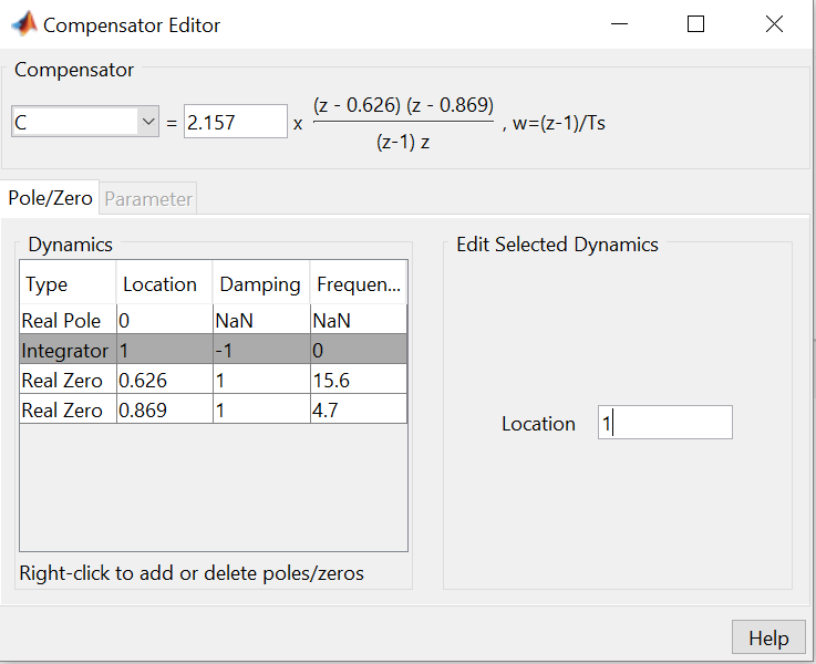
Open Edit Compensator to know the values you'll be using for the next steps.

NOTE: You should first go to the Control System Tab > Preferences. Once the Preferences window is open, go to the Options tab and mark Zero/Pole/Gain instead of whatever option is showed.

Figure 6. Edit Compensator showing all values we are interested on.