State-State Representation

clc
clear

% ---------- SYSTEM ---------- %
% numerator = [1 2.2];
% denominator = [1 -5.7 9];
% Gs = tf(numerator,denominator);
% fc = ;
% fs = fc*7;
% T = 2*pi/fs;
% Ts = round(T,2); % The sampling time must be rounded up (2 decimal places)
% Gz = c2d(Gs, Ts);
% kp_system = numerator(2)/denominator(3);

% ---------- STATE-SPACE REPRESENTATION ---------- %
sys = ss(Gz);

% Verify if the system is controllable
% The rank of controllability matrix should be that of the order of the
% system
%control_matrix = ctrb(sys.a, sys.b);
%rank_control_matrix = rank(control_matrix);

% Verify if the system is observable
% The rank of observability matrix should be that of the order of the
% system
%obsv_matrix = obsv(sys.a, sys.c);
%rank_obsv_matrix = rank(control_matrix);

% ---------- STATE FEEDBACK ---------- %
% The system is controllable, we can place poles wherever we want using a
% gain
% Remember you must place as many poles as the order of the system
ss_gain = acker(sys.a, sys.b, [0.7 0.8 0.75]);
open_loop_poles = eig(sys.a);
closed_loop_poles = eig(sys.a*sys.b-ss_gain);

% Matrix with the gain that places the poles on desired values
sys2 = ss(sys.a-sys.b*Gain, sys.b, sys.c, sys.d,T);
Gz2 = tf(Gz2);
% Obtain the final value in closed-loop of Gz2
% kp = ;

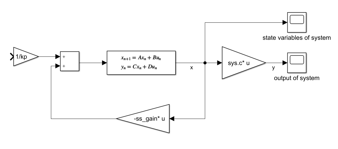
Simulink - State Feedback